Published 31 March 2020
Last updated on 2 April
The explanatory note that you can find here builds on joint work of:
Kristof Decock (FBS, MSI KU Leuven), Jorge Ricardo Blanco Nova (Institute of the Future, Rega Institute), Michela Bergamini (MSI, KU Leuven), Koenraad Debackere (KU Leuven, ECOOM), Sien Luyten (FBS), Xiaoyan Song (ECOOM, KU Leuven), Anne-Mieke Vandamme (Rega Institute, Institute of the Future) and Bart Van Looy (Dean FBS, MSI/KU Leuven, ECOOM).
Early 2020 the COVID-19 disease spread with an accelerated speed throughout Italy and then, almost equally hard, hit Spain. Epidemiologists and authorities are attempting to contain the spread of the disease on a global scale. We decided to step in with our knowledge and expertise.
In Flanders Business School we have been teaching foresight, forecasting and scenario thinking for decades. Maybe the diffusion models which we use to forecast the introduction of new products and services could be of use? Could scenario thinking be of any relevance?
We formed a transdisciplinary team of researchers from Flanders Business School, FEB (MSI & ECOOM) KU Leuven and Rega Institute/Institute of the Future (KU Leuven). Recently Anne Mieke Vandamme talked about our work on the VRT News:
We were particularly looking at the diffusion model of Bass, which descibes the adoption of new technologies by first-time buyers and how they influence other potential users who in their turn also contaminate further users and so on. Frank Bass, a professor at the Graduate School of Purdue University, developed his model more than 50 years ago. If you want to know more about his model, you can read Bass Re-visited, by Decock, Debackere & Van Looy (2020) which you find below.
Could it be that the spread of the virus would follow similar patterns? After all, diffusion curves are built on processes comparable to infection and inflammation.
Almost all diffusion models follow S-shaped curves as you see here:
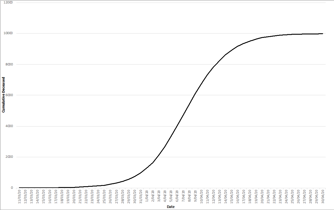
In our modelling exercise, m reflects the size of the population, or the size of the market. In this case – when modelling the COVID19 diffusion patterns – the m reflects the total number of deceased people.
Notice that we talk here about the cumulative number, which reflects an ‘end state’ after the first peak of the current pandemic is over.
Besides m, each curve also implies a p and a q parameter. Whereas the p parameter reflects the number of ‘inflammations’ (new cases introduced in a region/country from the outside), the q parameter reflects the intensity of contamination or infection (how many people become infected by a person who is contaminated).
How do we build models when time series are unfolding and we don’t know exactly what the end state will be?
Until now, most researchers focused on finding the ‘one best’ curve, that would predict both the near as well as the medium/long term future (end state). Decock, Debackere & Van Looy (2020) provide an overview of the state of the literature in this respect, and the conclusion that everyone seems to agree upon is that you cannot select an accurate path, based on data which only reflect the first part of the trajectory.
For instance, Van den Bulte and Lilien (1997, p. 350) concluded that “expecting a simple time series with a handful of noisy data points to foretell both the ultimate market size and the time path of market evolution is asking too much of too little data”. Whereas Mahajan et. al (1990, p.9) settle that “[…] parameter estimation for diffusion models is primarily of historical interest; by the time sufficient observations have developed for reliable estimation, it is too late to use the estimates for forecasting purposes”.
While we fully agree with this conclusion, it also inspired us to look at forecasting in a different way.
What if we would first sketch a landscape of all different (potential) paths, and then project also the actual, unfolding, data on the map depicting that landscape? Would the unfolding time series then not point into the direction of the end state?
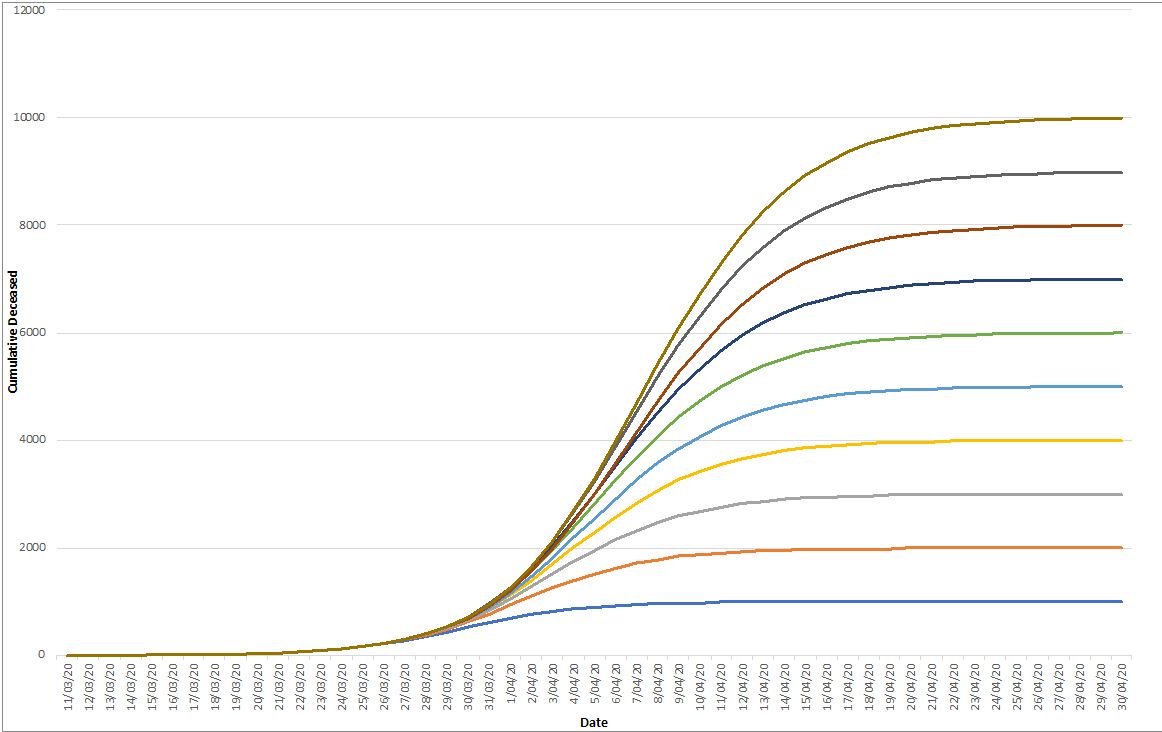
In order to create an exhaustive map, one needs calculation power. In total we explored 250 000 different combinations (all reflecting unique combinations of m, p & q). The boundaries of the landscape have been inspired by the size of the population for m and previous literature for the values for p and q.
Once we have calculated all these combinations, we select only those which are close to the unfolding time series.
In most cases, we have several hundred candidates of curves (each consisting of one unique set of the three parameters), all pointing to different end states (and with a different pace). So you might start to wonder, what can we do with such a wide range of potential trajectories and end states?
Well, now time has to do its job. We made such a map on March 25 with reported casualties for Belgium on that day (about a week ago). Then we wait for a few days to see how the actual numbers manifest themselves.
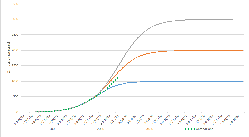
On March 30, we were looking at the following curve:
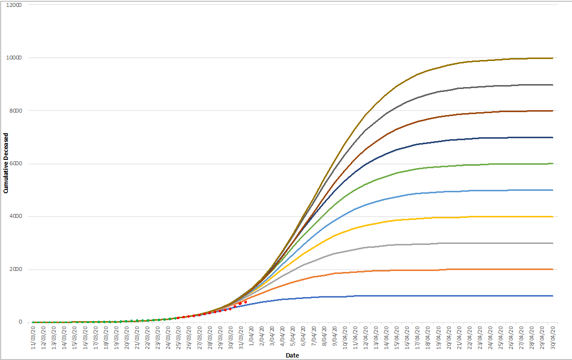
The green dots are observations that have been used to model the different end states. The red dots reflect the observations obtained afterwards.
Which tend us to conclude that the number of casualties in Belgium will be situated between the 1000 and 2000 curves.
Of course, which end state will materialize will depend critically on the impact of the ‘lock down’ measures that were taken on March 13. The coming days will be revealing in this respect and will be incorporated in daily updates of this forecasting note.
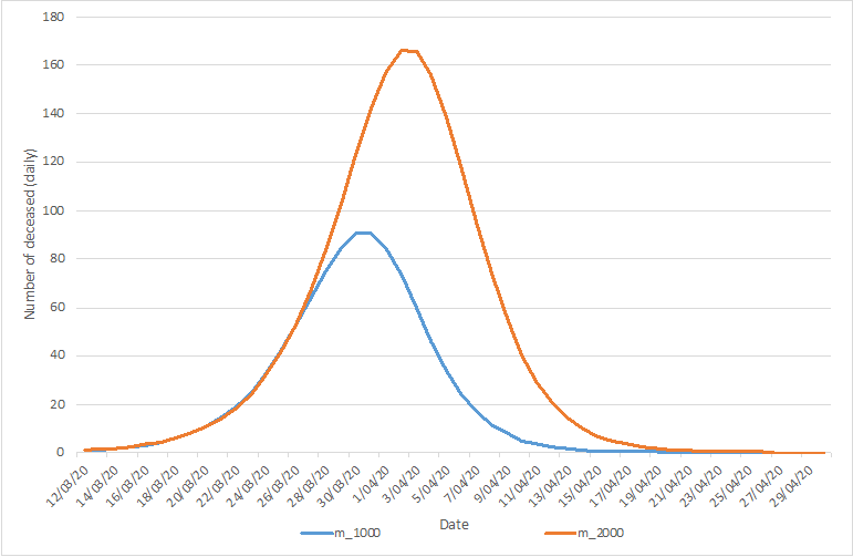
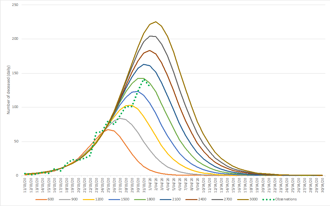
In the lower extreme scenario, 1.000 cumulative casualties are predicted, with an associated peak of daily casualties reaching 90 on March 30 and March 31 (the number reported by Sciensano for March 30 equaled 82, the number of March 31, 98 (excluding the additional 94, on which we comment below), after which a decline sets in. In the upper extreme scenario, 2.000 cumulative causalities are predicted, with an associated peak a few days later (April 3 & April 4) with a number around 165 during these two days. After that, the decline sets in.
These predictions are graphically depicted in the following figures.
To conclude:
Forecasts need foresight, and vice versa
Our approach departs from the traditional way of forecasting the future. Instead of looking for the ‘one and only’ future, we blend forecasting models with scenario oriented thinking.
By doing so, we provide simultaneously an insight in what is going on, when it will take place, and where it might lead us to.
Distance, not updates
One of the more striking insights of our research relates to distance. And by that, we don’t mean the physical/social distance that we started to redefine during recent weeks, but temporal distance. This approach only works well when you combine models of days (or even weeks) ago with actual observations. Recalculating the curves every day is useful to obtain a more precise picture of the days ahead. However, if you want to see what is beyond the horizon of next week, you’d better apply models which have been calibrated on older data.
PS: What if the underlying data are not accurate?
On March 31, Sciensano, the Belgian Federal Health Agency reported two numbers of deceased persons. One regular, relating to the deceased of the last 24 hours (n=98), and one additional, pertaining to 94 deceased people since March 11 not earlier accounted for.
Similar corrections have been reported on April 1 and April 2.
As a consequence, the initial time series - on which we built our first models and resulting graphs – changed significantly. For instance, the initial reported number of cumulative deceased people (in BE) for March 20 rose from 37 to 72. For the whole period of observations – which we use for our models - the numbers have been redefined upwards with a factor ranging between 3 (for the early days, when the cumulative numbers are still low) and 1.25/1.44 for more recent dates (end of March).
It goes without saying that changes in the underlying data affect the level of expected end states. While our initial models signaled end states between 1.000 and 1.200 casualties, the models that we recalculated on April 1 and April 2 signal more likely end states around 1.800 deceased. Take a look at the graphs below, and you notice that our predicted number of (reported) deceased would be 135 on April 3. The actual number reported for this day was 132. Also, the ‘predicted’ cumulative number of deceased (for Belgium) is very close to the reported numbers (we expected a range between 1085 and 1120 while the actual number is 1109).
As such, our models strongly suggest that we are currently at the peak of the pandemic for Belgium. Notice that we are about three weeks after the government took some drastic measures in terms of social distancing/gatherings etc. It looks like these measurements were and still are highly appropriate and needed in order to limit the number of casualties. These data are not just dots on a curve. They represent people who lost their lives. So be wise and stay out of these graphs!
A final disclaimer, if the numbers for March are going to be revised significantly upward (again), the validity of the curves that we depict here will no longer hold. If such revisions are occasional and minor (units) then we are confident our maps point into the right direction. Concretely, the number of people losing their lives through COVID-19 related health issues will be around 10 on April 13, and drop below 5 from 16 or 17 April onwards.
Read more about our work on the site of the Institute of the Future.
References
Bass, F.M. (1969). A New Product Growth for Model Consumer Durables. Management Science, 15 (5), 215-227.
Decock, K., Debackere, K. and Van Looy, B. (2020). Bass Re-visited: Quantifying Multi-Finality. MSI working paper, n° 2003.
Mahajan, V., Muller, E., and Bass, F.M. (1990). New product diffusion models in marketing: a review and directions for research. Journal of Marketing, 54 (1), 1-26.
Van den Bulte, C., and Lilien, G. L. (1997). Bias and systematic change in the parameter estimates of macro-level diffusion models. Marketing Science, 16, 338-353.